
On this page
Every vector database and every retrieval-augmented generation (RAG) system rests on one operation: given a query vector, find the stored vectors closest to it. With a few thousand vectors that is a loop. With tens of millions, comparing the query with every vector takes too long for an interactive request, so systems use approximate nearest neighbour (ANN) indexes that look at a small fraction of the data and accept that they will occasionally miss a true neighbour.
This article explains the algorithms behind those indexes as of August 2024: exact search, the inverted file index (IVF), product quantization (PQ) and the HNSW graph. It covers what each one does, which parameters control the trade-off between recall, speed and memory, and how to measure that trade-off on your own data. The sample code implements exact search, IVF and HNSW in plain NumPy so the parameters can be read and experimented with.
Exact search and the recall measure
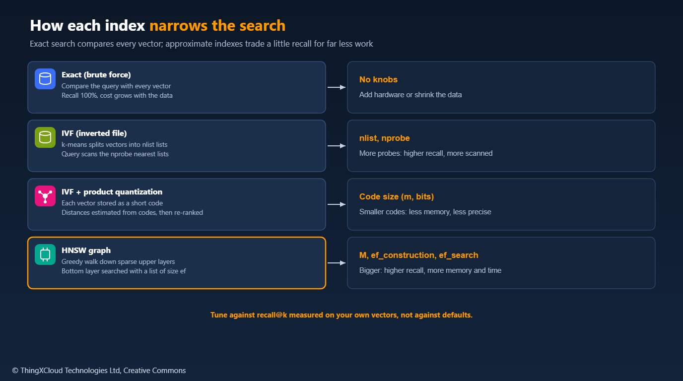
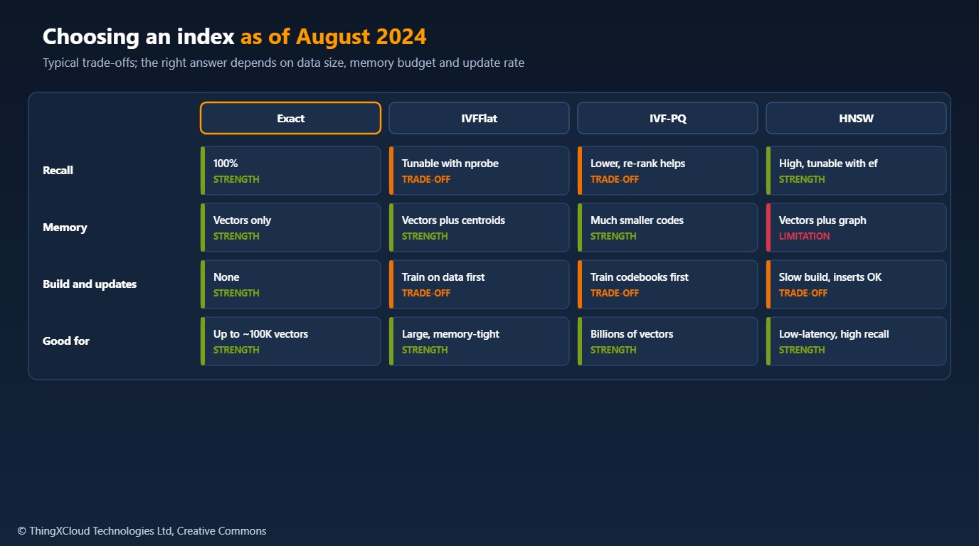
Exact search computes the distance from the query to every stored vector and keeps the k smallest. It is always correct and needs no index, which makes it the right choice for small collections and the reference for everything else. Approximate indexes are judged by recall@k: the share of the true k nearest neighbours, as found by exact search, that the index returns. Most production systems target recall between 0.9 and 0.99, chosen by how much a missed neighbour costs the application.
Distance choice matters less than it looks. For embeddings normalised to unit length, ranking by cosine similarity, by inner product and by Euclidean distance gives the same order, so normalise once and use whichever metric the index handles fastest.
IVF: search only the nearby partitions
An inverted file index runs k-means on the vectors to find nlist centroids and assigns every vector to its nearest centroid, producing nlist lists. At query time it finds the nprobe centroids nearest the query and scans only their lists. More lists make each list shorter; more probes raise recall and the amount scanned. A true neighbour is missed when it sits in a list just across a partition boundary that was not probed, which is why recall rises quickly with the first few extra probes.
IVF needs training data: build the index after loading a representative sample, not on an empty table, or the centroids will not reflect the data. pgvector’s documentation makes the same point about building IVFFlat indexes once the table has data.
Product quantization: compress the vectors
Product quantization, introduced by Jégou, Douze and Schmid, splits each vector into sub-vectors, runs k-means separately in each sub-space, and stores each vector as the list of nearest centroid IDs in each sub-space. A 768-dimensional float32 vector (3,072 bytes) can become a code of a few dozen bytes. Distances between a query and a code are estimated from small per-query lookup tables, which is fast. Combined with IVF (IVF-PQ), it lets a single machine search very large collections; the cost is lower precision, usually recovered by re-ranking the top candidates with their full vectors.
HNSW: navigate a graph
Hierarchical navigable small world graphs, described by Malkov and Yashunin, connect each vector to nearby vectors in a multi-layer graph. Each vector is placed in the bottom layer and, with exponentially decreasing probability, in higher layers, so the upper layers are sparse and act like express lanes. A query starts at the top, walks greedily towards the query until it cannot get closer, drops a layer and repeats, then searches the bottom layer keeping a candidate list of size ef.
%%{init: {'theme': 'base', 'themeVariables': {'primaryColor': '#FFF3E0', 'primaryTextColor': '#232F3E', 'primaryBorderColor': '#FF9900', 'lineColor': '#232F3E', 'clusterBkg': '#F8FAFC', 'clusterBorder': '#CBD5E1', 'edgeLabelBackground': '#FFFFFF', 'nodeTextColor': '#232F3E'}}}%%
flowchart TD
    A["Start at the entry point<br/>on the top layer"] --> B["Move to the neighbour<br/>closest to the query"]
    B --> C{"Any neighbour closer?"}
    C -- "Yes" --> B
    C -- "No" --> D{"Bottom layer?"}
    D -- "No" --> E["Drop one layer,<br/>start from the same node"]
    E --> B
    D -- "Yes" --> F["Search with a candidate<br/>list of size ef"]
    F --> G["Return the k closest"]
    classDef aws fill:#FFF3E0,stroke:#FF9900,stroke-width:2px,color:#232F3E
    classDef ok fill:#F0FFF4,stroke:#1D8102,stroke-width:2px,color:#145202
    class A,B,C,D,E,F aws
    class G ok
Three parameters matter. M is the number of links per node: higher values improve recall and use more memory. ef_construction is the candidate list size while building: higher values build a better graph more slowly. ef_search (often just ef) is the candidate list size at query time, the knob for recall against latency. In pgvector 0.7.0, for example, the defaults are m = 16, ef_construction = 64 and hnsw.ef_search = 40, and its documentation notes that HNSW has a better speed-recall trade-off than IVFFlat but builds more slowly and uses more memory.
The sample implements exact search, IVF and HNSW, with a recall function to compare them:
"""Three nearest-neighbour search algorithms in plain NumPy, for reading.

- `brute_force`: exact search; the reference every approximate index is
  measured against.
- `IVFFlat`: inverted file index. k-means splits the vectors into `nlist`
  clusters; a query scans only the `nprobe` closest clusters.
- `HNSW`: hierarchical navigable small world graph (Malkov and Yashunin).
  A query descends sparse upper layers greedily, then searches the dense
  bottom layer with a candidate list of size `ef`.
- `recall_at_k`: the share of the true k nearest neighbours an index returns.

Distances are squared Euclidean. For cosine similarity, normalise vectors to
unit length first; the ranking is then the same. Production libraries (FAISS,
hnswlib, the engines inside vector databases) are far faster; these versions
exist to make the parameters understandable.
"""
from __future__ import annotations

import heapq
import math

import numpy as np


def _sqdist(a: np.ndarray, b: np.ndarray) -> np.ndarray:
    return ((a - b) ** 2).sum(axis=-1)


def brute_force(data: np.ndarray, query: np.ndarray, k: int) -> np.ndarray:
    d = _sqdist(data, query)
    idx = np.argpartition(d, min(k, len(d) - 1))[:k]
    return idx[np.argsort(d[idx])]


def recall_at_k(found: np.ndarray, truth: np.ndarray) -> float:
    return len(set(found.tolist()) & set(truth.tolist())) / len(truth)


class IVFFlat:
    def __init__(self, nlist: int, iterations: int = 20, seed: int = 0):
        self.nlist, self.iterations = nlist, iterations
        self.rng = np.random.default_rng(seed)

    def fit(self, data: np.ndarray) -> "IVFFlat":
        if self.nlist > len(data):
            raise ValueError("nlist cannot exceed the number of vectors")
        self.data = data
        centroids = data[self.rng.choice(len(data), self.nlist, replace=False)].copy()
        for _ in range(self.iterations):                       # Lloyd's k-means
            assign = np.argmin(((data[:, None, :] - centroids[None, :, :]) ** 2).sum(-1), axis=1)
            for c in range(self.nlist):
                members = data[assign == c]
                if len(members):
                    centroids[c] = members.mean(axis=0)
        self.centroids = centroids
        self.lists = [np.flatnonzero(assign == c) for c in range(self.nlist)]
        return self

    def search(self, query: np.ndarray, k: int, nprobe: int = 1) -> np.ndarray:
        probe = np.argsort(_sqdist(self.centroids, query))[:nprobe]
        cand = np.concatenate([self.lists[c] for c in probe])
        if len(cand) == 0:
            return cand
        order = np.argsort(_sqdist(self.data[cand], query))[:k]
        return cand[order]

    def scanned(self, query: np.ndarray, nprobe: int) -> int:
        probe = np.argsort(_sqdist(self.centroids, query))[:nprobe]
        return int(sum(len(self.lists[c]) for c in probe))


class HNSW:
    def __init__(self, M: int = 16, ef_construction: int = 100, seed: int = 0):
        if M < 2:
            raise ValueError("M must be at least 2")
        self.M, self.M0, self.efc = M, 2 * M, ef_construction
        self.mL = 1 / math.log(M)
        self.rng = np.random.default_rng(seed)
        self.vectors: list[np.ndarray] = []
        self.graph: list[dict[int, list[int]]] = []    # graph[layer][node] -> neighbours
        self.entry: int | None = None
        self.top = -1

    def _d(self, i: int, q: np.ndarray) -> float:
        return float(((self.vectors[i] - q) ** 2).sum())

    def _search_layer(self, q: np.ndarray, entries: list[int], ef: int, layer: int) -> list[tuple[float, int]]:
        visited = set(entries)
        cand = [(self._d(e, q), e) for e in entries]
        heapq.heapify(cand)                                    # closest first
        best = [(-d, e) for d, e in cand]                      # farthest first (max-heap)
        heapq.heapify(best)
        while cand:
            d, c = heapq.heappop(cand)
            if d > -best[0][0] and len(best) >= ef:
                break
            for n in self.graph[layer].get(c, []):
                if n in visited:
                    continue
                visited.add(n)
                dn = self._d(n, q)
                if len(best) < ef or dn < -best[0][0]:
                    heapq.heappush(cand, (dn, n))
                    heapq.heappush(best, (-dn, n))
                    if len(best) > ef:
                        heapq.heappop(best)
        return sorted((-d, e) for d, e in best)

    def add(self, v: np.ndarray) -> int:
        node = len(self.vectors)
        self.vectors.append(np.asarray(v, dtype=float))
        level = int(-math.log(1.0 - self.rng.random()) * self.mL)
        while len(self.graph) <= level:
            self.graph.append({})
        for layer in range(level + 1):
            self.graph[layer][node] = []
        if self.entry is None:
            self.entry, self.top = node, level
            return node
        ep = [self.entry]
        for layer in range(self.top, level, -1):              # greedy descent
            ep = [self._search_layer(v, ep, 1, layer)[0][1]]
        for layer in range(min(level, self.top), -1, -1):
            found = self._search_layer(v, ep, self.efc, layer)
            cap = self.M0 if layer == 0 else self.M
            neighbours = [e for _, e in found[: self.M]]
            self.graph[layer][node] = neighbours
            for n in neighbours:                               # connect both ways, then prune
                links = self.graph[layer][n]
                links.append(node)
                if len(links) > cap:
                    links.sort(key=lambda x: self._d(x, self.vectors[n]))
                    del links[cap:]
            ep = [e for _, e in found]
        if level > self.top:
            self.entry, self.top = node, level
        return node

    def fit(self, data: np.ndarray) -> "HNSW":
        for v in data:
            self.add(v)
        return self

    def search(self, q: np.ndarray, k: int, ef: int = 50) -> np.ndarray:
        if self.entry is None:
            return np.array([], dtype=int)
        ep = [self.entry]
        for layer in range(self.top, 0, -1):
            ep = [self._search_layer(q, ep, 1, layer)[0][1]]
        found = self._search_layer(q, ep, max(ef, k), 0)
        return np.array([e for _, e in found[:k]])
Measuring the trade-off
The sample’s example.py runs both indexes on 2,000 synthetic 32-dimensional vectors in 16 clusters and compares their results with exact search. The figures describe this toy data and these simple implementations, not any product, but they show the shape of the trade-off:
| Index and setting | Recall@10 | Work per query |
|---|---|---|
| IVF, nlist 32, nprobe 1 | 0.875 | 114 vectors scanned |
| IVF, nlist 32, nprobe 2 | 0.953 | 203 vectors scanned |
| IVF, nlist 32, nprobe 4 | 0.993 | 302 vectors scanned |
| IVF, nlist 32, nprobe 8 | 1.000 | 577 vectors scanned |
| HNSW, M 12, ef 10 | 0.978 | graph walk |
| HNSW, M 12, ef 100 | 0.980 | graph walk |
Do the same with your embeddings and a few hundred real queries: compute exact neighbours once, then sweep nprobe or ef_search and plot recall against latency. Pick the cheapest setting that meets your recall target, and measure again when the data grows or the embedding model changes.
A query with a metadata filter (tenant, date, language) applied after the approximate search can return fewer than k results, or miss neighbours that the filter would have kept. Check how your database combines filters with the index, raise ef_search or nprobe for filtered queries, or use exact search when a filter selects a small subset.
Retrieve more candidates than you need from the approximate index (say 50 for a final 10), then re-rank them with full-precision distances or a cross-encoder. It recovers most of the recall lost to compression and costs little because the candidate set is small.
Vectors, product-quantization codes and graph links are derived from the source documents and can leak information about them. Apply the same access control, encryption and deletion rules to vector indexes as to the documents, and make sure a deletion request removes the vector from every index and replica.
ann.py was tested with Python 3.12, numpy==1.26.4 and pytest==8.3.2: six tests cover exact search, IVF returning exact results when every list is probed, IVF recall rising with nprobe while scanning under half the data, HNSW recall of at least 0.95 rising with ef, HNSW degree limits and layers, and parameter validation. The table is the output of the sample’s example.py. pgvector defaults are from its 0.7.0 documentation.
Key takeaways
- Exact search is correct and simple; it is the baseline and often enough for small collections.
- IVF partitions with k-means and scans the nprobe nearest lists; it needs training data and is memory-light.
- Product quantization compresses vectors into short codes for very large collections; re-rank to recover precision.
- HNSW gives high recall at low latency, at the cost of memory and build time; tune ef_search for recall.
- Measure recall@k against exact search on your own vectors and queries, including filtered queries.
Which index and settings did you settle on, and what recall do you measure in production? Share it in the comments.
The complete sample for this article is on GitHub: nithinmohantk/blog-samples-working-repo/ann-algorithms. Clone it with git clone https://github.com/nithinmohantk/blog-samples-working-repo.git and open the ann-algorithms folder. Its README says how to run it and what has been verified.
Glossary
- ANN
- Approximate nearest neighbour search: finding close vectors without comparing against all of them.
- Recall@k
- The share of the true k nearest neighbours that a search returns.
- IVF
- Inverted file index: vectors grouped into lists by nearest k-means centroid.
- nprobe
- The number of IVF lists searched per query.
- Product quantization
- Compressing vectors into codes of per-sub-space centroid IDs.
- HNSW
- Hierarchical navigable small world: a layered proximity graph searched greedily.
- ef_search
- HNSW query-time candidate list size; higher means better recall and slower queries.
References & Further Reading
- → Efficient and robust approximate nearest neighbor search using HNSW graphs— Malkov and Yashunin: the HNSW paper
- → Product Quantization for Nearest Neighbor Search— Jégou, Douze and Schmid, IEEE TPAMI 2011
- → pgvector 0.7.0— HNSW and IVFFlat options and defaults in PostgreSQL
- → Sample code for this article— Exact search, IVF and HNSW in NumPy with recall measurement
Discover more from C4: Container, Code, Cloud & Context
Subscribe to get the latest posts sent to your email.
